A processor can run a neural network on very little energy and still deliver only modest savings for the device using it. The camera, data preparation, or supporting computer may consume much more than the computation. That boundary between the chip and the system determines much of the value of neuromorphic computers.
Neuromorphic computers incorporate principles of neural processing into electronic architectures: distributed state, memory close to computation, and, in many designs, communication through events. They run artificial intelligence algorithms. Their distinction lies in how they organize work and move information, rather than in possessing a form of intelligence separate from AI.
Evaluating them requires examining three different implementations: Loihi 2/Hala Point, NorthPole, and BrainScaleS-2. The cited sources were available by October 27, 2026. Numerical examples labeled as educational are illustrative calculations, not measurements of those devices.
What a silicon neuron actually computes
In a spiking neural network, or SNN, a neuron maintains internal variables and receives events from other neurons. A simple model integrates contributions and emits a spike when it crosses a threshold. Timing matters: two closely spaced inputs may produce an output that would not occur if they arrived far enough apart.
An educational example of leaky integration uses this update: next u = 0.9 × previous u + sum of weighted inputs. If the result reaches 1, the neuron emits a spike and subtracts 1 from its state. These dynamics and reset are teaching choices; they do not describe every chip.
Starting with a state of 0.6 and inputs totaling 0.3, the first result is 0.84: no spike. If the next step receives another 0.3, the state reaches 1.056, emits a spike, and remains at 0.056. Short-term memory resides in the state that persists between inputs.
This example separates three engineering decisions: how long memory lasts, when a result is communicated, and how much activity that communication generates. Changing any of them can affect accuracy and cost. Counting neurons without specifying their dynamics leaves part of the problem out of view.
Local memory helps; traffic still has a cost
Accelerating an arithmetic operation is not enough in a distributed application. The system must also access weights and move results. The architectural opportunity is to keep state close to where it is used and avoid movements that contribute no useful information.
The Loihi 2 technical brief describes 128 neuromorphic cores, programmable neuron models, and configurable learning rules. Messages can carry graded values; communication is not restricted to identical binary spikes.
The practical consequence is that the same neuron count can produce very different workloads. A neuron sending its output to many destinations creates more distribution work. If connections frequently cross chip boundaries, network placement and communication queues become part of performance.
Three architectures that need separate assessments
| Implementation | Relevant characteristic | Evaluation question |
|---|---|---|
| Loihi 2 / Hala Point | Digital spiking networks and distributed state | How is the model distributed, and how much traffic does it generate? |
| NorthPole | Inference with computation and memory integrated on-chip | Does the model fit, and what does the complete task cost? |
| BrainScaleS-2 | Accelerated analog neural dynamics with digital control | How do calibration and variability affect the experiment? |
Loihi 2 and Hala Point: scaling also requires communication
Intel introduced Hala Point in 2024 with 1,152 Loihi 2 processors and capacity for 1.15 billion artificial neurons. It specified maximum power consumption of 2,600 W. These are system specifications, not energy per classification or a statement of cognitive equivalence to a brain.
Our recommendation when selecting a platform is to request the application's actual configuration. Installed capacity and real utilization answer different questions. A network fitting in memory may still encounter a limit in its connectivity or the time available to process each input.
NorthPole: brain inspiration without requiring an SNN
The IBM paper published in Science in 2023 integrates memory and computation for inference. On ResNet50, compared with a GPU using a comparable 12 nm manufacturing process, it reported 25 times more frames per second per watt and 22 times lower latency.
That result must retain its task and reference. It does not transfer the factor of 25 to every model or establish a direct comparison with a newer GPU. NorthPole illustrates a useful distinction: brain-inspired computing is a broader family than spiking networks. A commercial label alone does not identify the mechanism.
BrainScaleS-2: faster dynamics do not make everything faster
The 2022 BrainScaleS-2 paper describes analog neuron circuits and digital processors for plasticity. The dynamics operate approximately a thousand times faster than their biological reference. This accelerates a physical model; it does not promise to run every program a thousand times faster.
Experimental design must also budget for preparation, input, and reading results. Compressing circuit time makes supplying and observing it more demanding. The useful measurement is complete execution time, including necessary calibration, rather than the neural timescale alone.
Training, inference, and adaptation are different jobs
Inference produces an output using an already configured model. Training changes its parameters. Adaptation during use adds another requirement: deciding what to update with new data without destroying earlier learning. A device efficient at one of these jobs does not automatically demonstrate the others.
Spiking networks can be trained through different procedures. The surrogate gradient paper by Neftci, Mostafa, and Zenke explains how learning can approximate the problematic derivative of a spike. Using spikes during execution therefore does not imply eliminating numerical optimization or external training.
Before a pilot, I would request an explicit cost breakdown: what is trained outside the chip, which parameters can change inside it, and what information the update requires. It is also worth asking whether learning continues when correct labels disappear. Learning with supervision available differs from adapting without it.
An October 2026 result and what it excludes
The CLP-SNN preprint, revised October 20, 2026, reports a prediction-and-update step on Loihi 2 taking 0.33 ms and 0.05 mJ on extracted features. The comparison excludes feature extraction and host communication; its 25-shot protocol achieves 90.0% accuracy.
Our proposed reading separates that step's benefit from the complete product's performance. An application that must first produce those features needs to measure that additional work. Differences should not all be attributed to chip manufacturing when algorithms and numerical precision also change. A preprint provides examinable evidence, rather than independent certification.
Input can preserve or erase the advantage
The event-based vision survey by Gallego and colleagues describes cameras that communicate per-pixel brightness changes with position, time, and sign. That output differs from a sequence of complete images at a fixed frame rate.
As a design example, imagine a camera monitoring an item crossing a conveyor belt. The aim is to detect relevant changes and respond within a deadline. A pipeline preserving events may avoid constructing intermediate images that it would later transform again. The advantage must be tested with real movement and lighting.
If software accumulates events in long windows, it may introduce a delay incompatible with the required response. Vibration or flicker generating abundant activity changes the input rate. Our proposed test would include both extremes alongside the comfortable scenario with little activity.
Measuring energy without hiding the rest of the device
For an engineering assessment, we propose this balance: total energy = sensor + data preparation + processor + communication + supporting equipment. Define where measurement starts and ends, and use the same boundary for alternatives. Manufacturer-rated maximum power cannot replace that measurement.
A hypothetical example: a complete operation consumes 100 mJ, with 90 spent by the rest of the equipment and 10 by the processor. Cutting those 10 to 1 mJ reduces processor energy tenfold. Total energy falls to 91 mJ: the system saves 9%. The arithmetic explains why a striking chip improvement may have a small product-level effect.
Useful energy also depends on output quality. I recommend counting correct decisions delivered within the deadline, reporting errors, and separating idle consumption from consumption during activity. A lower-energy detector that frequently raises false alarms is solving a different problem from the one required.
A comparison protocol that supports a decision
NeuroBench, published in 2025, distinguishes algorithm evaluation from system evaluation. That separation helps identify whether an improvement comes from the model or its implementation. For a specific pilot, we propose agreeing on these conditions before running the demonstration:
| Condition | What to record | What it prevents |
|---|---|---|
| Equivalent quality | Accuracy and false positives on the same held-out data | Comparing savings obtained by doing the task worse |
| Complete response | Input-to-decision time; 50th and 99th percentiles | Hiding queues and delays behind an average |
| Common energy boundary | Included components, idle energy, and energy per operation | Comparing an isolated chip with an entire device |
| Representative workload | Low activity, bursts, noise, and saturation | Showing only the favorable scenario |
| Integration cost | Model conversion, memory, tooling, and engineering time | Confusing a laboratory demonstration with a ready product |
The reference should include a well-tuned conventional implementation appropriate to the workload. For a small sensor, comparison with a microcontroller or integrated NPU may be more informative than comparison with a data-center GPU. Choosing an oversized reference makes a headline easier but gives poor purchasing guidance.
Technical questions before choosing a neuromorphic computer
Is an SNN running on a GPU already neuromorphic hardware?
No. The model uses spikes; the GPU retains its architecture. Judging efficiency requires measuring the implementation that actually runs.
Does a million neurons specify how many parameters fit?
Not by itself. Connectivity, precision, state variables, and memory limits matter. Those constraints may determine which model actually fits.
Does memory near computation eliminate transfers?
Inputs, outputs, and communication between units remain. The useful question is which transfers are reduced and which still dominate total cost.
Does local learning mean general autonomous learning?
No. A rule can update connections using local signals while still needing objectives, supervision, or rewards defined for a particular task.
Does an image benchmark advantage establish a language-model advantage?
No. Computational structure, memory requirements, and evaluation change. Each move to a different application needs its own demonstration.
Do these devices contain living neurons?
The three platforms described use electronics. Neural inspiration does not turn circuits into biological tissue or establish consciousness.
Where a pilot is worth starting
Our proposal is to prioritize pilots involving temporal signals, response constraints, and a measurable energy boundary: change detection, sensory processing, or bounded adaptation. These are not guaranteed advantages. They are conditions that allow a hypothesis to be formulated and rejected if the complete system fails to improve.
At the Laboratory of the Future, we follow how AI changes scientific work. For neuromorphic computers, adoption should be equally concrete: a defined task, comparable results, and an improvement that survives the move from the chip into the device someone will actually use.